
运行环境:WIN10 tensorflow1.3.1 CUDA10 python3.7 Keras Numpy matplotlib OpenCV
原程序来自于github:https://github.com/himanshurawlani/convnet-interpretability-keras
实现效果:卷积核可视化、热区图、中间激活层可视化、反卷积可视化
主要作用其实就是把卷积神经网络中的权重激活可视化的展现出来,最初提出具体请看这一篇论文
Grad-CAM: Visual Explanations from Deep Networks via Gradient-based Localization https://arxiv.org/abs/1610.02391
请教了一下计算机的同学,意思大概是Grad-CAM模型的优势在于不需要重新进行训练,在输出的时候不影响其权重的传递,不改变模型结构,可以直接输出。至于为什么用这一套代码,第一有注释非常清晰……第二我去找了原来论文的代码,不是基于tensorflow环境下的……不好运行,还有一些老的代码(16、17年左右的)在新环境下跑不出来总是报错,其他的一些代码也是需要caffe之类的,这个只需要tensorflow下的一些就可以。这个轮子非常好用!
论文的摘要:
我们提出了一种技术,用于为大量基于CNN的模型的决策产生“视觉解释”,使其更加透明。我们的方法 - 梯度加权类激活映射(Grad-CAM),使用任何目标概念的梯度,流入最终卷积层以生成粗略定位图,突出显示图像中的重要区域以预测概念。与以前的方法不同,GradCAM适用于各种CNN模型系列:(1)具有完全连接层的CNN(例如VGG),(2)用于结构化输出的CNN(例如字幕),(3)用于的CNN具有多模式输入(例如VQA)或强化学习的任务,无需任何架构更改或重新培训。我们将GradCAM与细粒度可视化相结合,以创建高分辨率的类辨别可视化,并将其应用于现成的图像分类,字幕和视觉问答(VQA)模型,包括基于ResNet的架构。在图像分类模型的背景下,我们的可视化(a)为他们的失败模式提供了见解(表明看似不合理的预测具有合理的解释),(b)对对抗性图像具有鲁棒性,(c)优于以前的弱监督定位方法,(d)更忠实于基础模型,(e)通过识别数据集偏差来帮助实现泛化。对于字幕和VQA,我们的可视化显示即使是非基于注意力的模型也可以本地化输入。最后,我们进行人体研究以衡量GradCAM解释是否有助于用户建立对深度网络预测的信任,并表明GradCAM帮助未经训练的用户成功地从“弱”的网络中辨别出“更强大”的深层网络。我们的代码可在 这个https网址。可以在此http URL和此http URL找到演示和演示视频。
具体怎么部署tensorflow环境和CUDA加速之类的,请看这篇文章:
WIN10+CUDA10 +CUDNN7.5+ TENSORFLOW-GPU1.13.1 + python3.7 运行NVIDIA STYLEGAN 的安装过程和踩坑实录
运行教程:这套代码使用需要不少运行的环境和包
所以嘛,先打开Anaconda pormpt
激活环境
activate tensorflow-gpu
输入pip命令安装这些包(因为我也不确定之前安装了什么,有可能不止这些,如果有报错可以再安装缺乏的包)
pip install opencv-python
pip install matplotlib
pip install Keras
然后打开adaconda,进入tensorflow-gpu环境,进入jupyter notebook 点击lunch

进入jupyter编辑器,打开刚刚下载并且解压的文件目录,打开heatmap_visualization_using_gradcam.ipynb
之后依次运行每一个程序块,注意,当左边[]括号里面有*的时候是正在运行,所以要等第一个执行完再执行下一个,不然会报错。在执行第一个的时候,可能会下载一个较大的(500M)预训练集,我感觉是下载到tensorflow的目录里面了,速度慢的话建议挂梯子。
下面是对这个程序内容的解释和翻译:
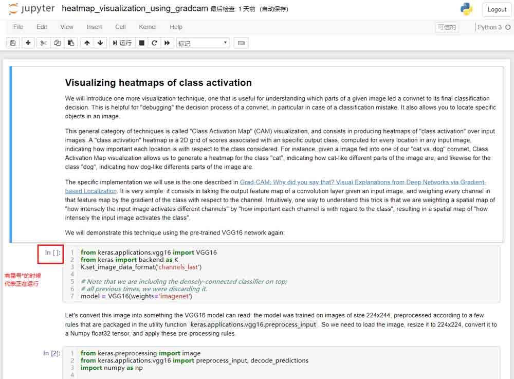
Visualizing heatmaps of class activation
We will introduce one more visualization technique, one that is useful for understanding which parts of a given image led a convnet to its final classification decision. This is helpful for "debugging" the decision process of a convnet, in particular in case of a classification mistake. It also allows you to locate specific objects in an image.
This general category of techniques is called "Class Activation Map" (CAM) visualization, and consists in producing heatmaps of "class activation" over input images. A "class activation" heatmap is a 2D grid of scores associated with an specific output class, computed for every location in any input image, indicating how important each location is with respect to the class considered. For instance, given a image fed into one of our "cat vs. dog" convnet, Class Activation Map visualization allows us to generate a heatmap for the class "cat", indicating how cat-like different parts of the image are, and likewise for the class "dog", indicating how dog-like differents parts of the image are.
The specific implementation we will use is the one described in Grad-CAM: Why did you say that? Visual Explanations from Deep Networks via Gradient-based Localization. It is very simple: it consists in taking the output feature map of a convolution layer given an input image, and weighing every channel in that feature map by the gradient of the class with respect to the channel. Intuitively, one way to understand this trick is that we are weighting a spatial map of "how intensely the input image activates different channels" by "how important each channel is with regard to the class", resulting in a spatial map of "how intensely the input image activates the class".
We will demonstrate this technique using the pre-trained VGG16 network again:
可视化类激活的热图
我们将介绍另一种可视化技术,这种技术有助于理解给定图像的哪些部分引导其进行最终的分类决策。这有助于“调试”回转网的决策过程,特别是在分类错误的情况下。它还允许您在图像中查找特定对象。
这种一般类别的技术称为“类激活图”(CAM)可视化,并且包括在输入图像上产生“类激活”的热图。“类激活”热图是与特定输出类相关联的分数的2D网格,针对任何输入图像中的每个位置计算,指示每个位置相对于所考虑的类的重要程度。例如,如果将图像输入我们的“猫与狗”之一,则类激活图可视化允许我们为类“猫”生成热图,指示图像中猫的不同部分是如何的,同样如此对于“狗”类,表示图像的狗状不同部分。
我们将使用的具体实现是Grad-CAM中描述的实现:你为什么这么说?深度网络中基于梯度的本地化的可视化解释。它非常简单:它包括在给定输入图像的情况下获取卷积层的输出特征图,并通过类相对于通道的梯度对该特征图中的每个通道进行加权。直觉上,理解这一技巧的一种方法是,我们通过“每个通道对于类别的重要程度”来加权“输入图像激活不同通道的强度”的空间图,从而产生“多么强烈的空间图”。输入图像激活类“。
我们将再次使用预先培训的VGG16网络演示此技术:
Let's convert this image into something the VGG16 model can read: the model was trained on images of size 224x244, preprocessed according to a few rules that are packaged in the utility function keras.applications.vgg16.preprocess_input. So we need to load the image, resize it to 224x224, convert it to a Numpy float32 tensor, and apply these pre-processing rules.
让我们将这个图像转换为VGG16模型可以读取的内容:模型在大小为224x244的图像上进行训练,根据实用函数中包含的一些规则进行预处理keras.applications.vgg16.preprocess_input。所以我们需要加载图像,将其大小调整为224x224,将其转换为Numpy float32张量,并应用这些预处理规则。
from keras.applications.vgg16 import preprocess_input, decode_predictions
import numpy as np# The local path to our target image
img_path = 'elephant.jpg'# `img` is a PIL image of size 224x224
img = image.load_img(img_path, target_size=(224, 224))# `x` is a float32 Numpy array of shape (224, 224, 3)
x = image.img_to_array(img)# We add a dimension to transform our array into a "batch"
# of size (1, 224, 224, 3)
x = np.expand_dims(x, axis=0)# Finally we preprocess the batch
# (this does channel-wise color normalization)
x = preprocess_input(x)
preds = model.predict(x)
print('Predicted:', decode_predictions(preds, top=3)[0])
Predicted: [('n02504458', 'African_elephant', 0.91017425), ('n01871265', 'tusker', 0.085445531), ('n02504013', 'Indian_elephant', 0.0043368866)]
The top-3 classes predicted for this image are:
African elephant (with 92.5% probability)
Tusker (with 7% probability)
Indian elephant (with 0.4% probability)
Thus our network has recognized our image as containing an undetermined quantity of African elephants. The entry in the prediction vector that was maximally activated is the one corresponding to the "African elephant" class, at index 386:
预测此图片的前三名是:
非洲象(概率为92.5%)
Tusker(概率为7%)
印度象(概率为0.4%)
因此,我们的网络已经认识到我们的形象包含一定数量的非洲大象。最大激活的预测向量中的条目是对应于“非洲大象”类的条目,在索引386处:
preds.shape
(1, 1000)
np.argmax(preds[0])
386
To visualize which parts of our image were the most contributing to the output, let's set up the Grad-CAM process:
为了可视化我们图像的哪些部分对输出的贡献最大,让我们设置Grad-CAM过程:
layer_names = ['block1_conv1', 'block1_conv2',
'block2_conv1', 'block2_conv2',
'block3_conv1', 'block3_conv2', 'block3_conv3',
'block4_conv1', 'block4_conv2', 'block4_conv3',
'block5_conv1', 'block5_conv2', 'block5_conv3']# This is the entry in the prediction vector
pred_vector_output = model.output[:, 386]heatmap = []
for layer_name in layer_names:
# The is the output feature map of the given layer, in VGG16
some_conv_layer = model.get_layer(layer_name)# This is the gradient of the predicted class with regard to
# the output feature map of selected block
grads = K.gradients(pred_vector_output, some_conv_layer.output)[0]# This is a vector of shape (512,), where each entry
# is the mean intensity of the gradient over a specific feature map channel
pooled_grads = K.mean(grads, axis=(0, 1, 2))# This function allows us to access the values of the quantities we just defined:
# `pooled_grads` and the output feature map of `block5_conv3`,
# given a sample image
iterate = K.function([model.input], [pooled_grads, some_conv_layer.output[0]])# These are the values of these two quantities, as Numpy arrays,
# given our sample image of two elephants
pooled_grads_value, conv_layer_output_value = iterate([x])# We multiply each channel in the feature map array
# by "how important this channel is" with regard to the elephant class
for i in range(model.get_layer(layer_name).output_shape[-1]):
conv_layer_output_value[:, :, i] *= pooled_grads_value[i]# The channel-wise mean of the resulting feature map
# is our heatmap of class activation
heatmap.append(np.mean(conv_layer_output_value, axis=-1))
len(heatmap)
13
from matplotlib import pyplot as plt
%matplotlib inline
For visualization purpose, we will also normalize the heatmap between 0 and 1:
出于可视化目的,我们还将热图在0和1之间标准化:
plt.figure(figsize=(18, 18))
for i in range(13):
plt.figure(figsize=(40,40))
plt.subplot(5, 3, i+1)
img_heatmap = np.maximum(heatmap[i], 0)
img_heatmap /= np.max(img_heatmap)
plt.imshow(img_heatmap)
plt.title(layer_names[i])
plt.show()
Finally, we will use OpenCV to generate an image that superimposes the original image with the heatmap we just obtained:
最后,我们将使用OpenCV生成一个图像,将原始图像与我们刚刚得到的热图叠加:
import cv2
# We use cv2 to load the original image
img = cv2.imread(img_path)
for i, hm in enumerate(heatmap):
img_heatmap = np.maximum(hm, 0)
img_heatmap /= np.max(img_heatmap)# We resize the heatmap to have the same size as the original image
img_hm = cv2.resize(img_heatmap, (img.shape[1], img.shape[0]))# We convert the heatmap to RGB
img_hm = np.uint8(255 * img_hm)# We apply the heatmap to the original image
img_hm = cv2.applyColorMap(img_hm, cv2.COLORMAP_JET)# 0.4 here is a heatmap intensity factor
superimposed_img = img_hm * 0.4 + img# Save the image to disk
cv2.imwrite('./elephant_{}.jpg'.format(layer_names[i]), superimposed_img)
plt.figure(figsize=(16, 16))
layer_name = 'input_image'
img = image.img_to_array(
image.load_img('./elephant.jpg')) / 255.
plt.imshow(img)
plt.title(layer_name)Text(0.5,1,'input_image')
plt.figure(figsize=(16, 16))
layer_name = 'block5_conv3'
img = image.img_to_array(
image.load_img('./elephant_{}.jpg'.format(layer_name))) / 255.
plt.imshow(img)
plt.title(layer_name)
Text(0.5,1,'block5_conv3')
plt.figure(figsize=(16, 16))
layer_name = 'block5_conv3'
img = image.img_to_array(
image.load_img('./elephant_{}.jpg'.format(layer_name))) / 255.
plt.imshow(img)
plt.title(layer_name)
Text(0.5,1,'block5_conv3')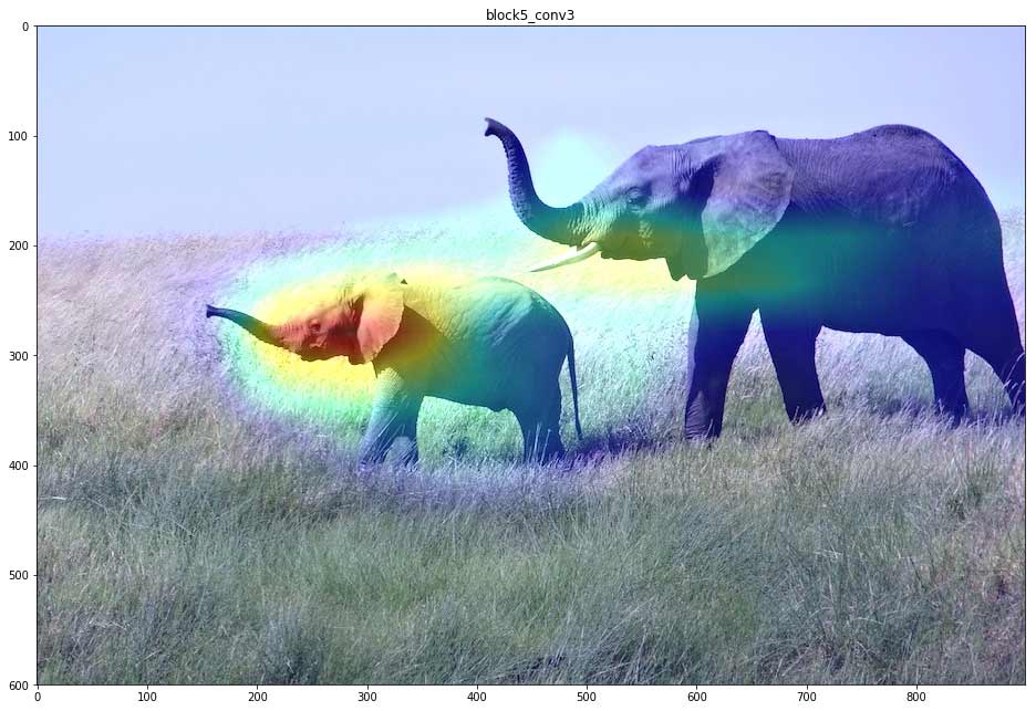
This visualisation technique answers two important questions:
Why did the network think this image contained an African elephant?
Where is the African elephant located in the picture?
In particular, it is interesting to note that the ears of the elephant cub are strongly activated: this is probably how the network can tell the difference between African and Indian elephants.
这种可视化技术回答了两个重要的问题:
为什么网络认为这张照片里有一头非洲象?
非洲象在图片中的位置是什么?
特别值得注意的是,幼象的耳朵被强烈地激活了:这可能是这个网络分辨非洲象和印度象的方式。


